Next: polalm
Up: GLESP Description and Examples
Previous: ntot
Description
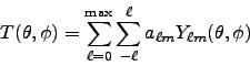
polmap synthesizes CMB temperature and polarization
maps from
spherical harmonic coefficients  and polarization mode coefficients
 and
and  .
.
 |
(6) |
To synthesize a map,
polmap
can process an file either in FITS Binary Extension-like or
in ASCII format, or can read
an ASCII string of .
If the input is a power spectrum  or
or  (where the ASCII
data have
to be in units of
(where the ASCII
data have
to be in units of  , and unitless),
polmap generates
a Gaussian map of CMB anisotropies by assigning
the = COMPLEX(
, and unitless),
polmap generates
a Gaussian map of CMB anisotropies by assigning
the = COMPLEX( ,
,  ) mutually independent Gaussian-distributed
real () and imaginary part (), both with a standard
deviation
) mutually independent Gaussian-distributed
real () and imaginary part (), both with a standard
deviation
 at each
  harmonic.
To synthesize polarization maps of Stokes-parameters Q and U,
polmap
can process 3-alm file containing , and data, separate
and files and file either
in FITS Binary Extension-like or
in ASCII format, or can read
an ASCII strings of and .
Maps of the Stokes parameters  and
and  are calculated with the potentials
 and
and  as follows:
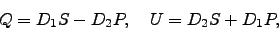 |
(7) |
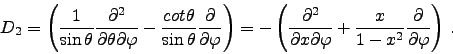
and operators  and
and  are:
are:
 |
(8) |
where  .
.
![\begin{displaymath}
S={1\over\sqrt{2\pi}}\sum_{l=2}^{l_{max}}\left(s_{l0}
f^0_l(...
...(x)[s_{lm}^c\cos(m\varphi)-
s_{lm}^s\sin(m\varphi)]\right) ,
\end{displaymath}](img56.png) |
(9) |
![\begin{displaymath}
P={1\over\sqrt{2\pi}}\sum_{l=2}^{l_{max}}\left(
f^0_l(x)+2\s...
...(x)[p_{lm}^c\cos(m\varphi)-
p_{lm}^s\sin(m\varphi)]\right) ,
\end{displaymath}](img57.png) |
(10) |
 |
(11) |
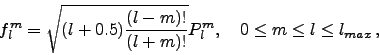
Here  and
and  are the associated Legendre
functions (ordinary and normalized) and
are the associated Legendre
functions (ordinary and normalized) and  and
and
 (of B and E-modes) are the coefficients of decomposition
characterizing properties of polarization.
See other details in the correpsnoding paper of GLESP 2.0.
(of B and E-modes) are the coefficients of decomposition
characterizing properties of polarization.
See other details in the correpsnoding paper of GLESP 2.0.
Examples
- Synthesizing an anisotropy map from given spherical harmonic
coefficients (-a, -as)
-
polmap -a alm.fits -t map.fits -nx 250 -np 500 -lmax 100
synthesizes the map from input FITS file 'alm.fits' and writes to the
file '
map.fits' with resolution (250,500). The maximum multipole
number is 100.
-
polmap -as "2,1,1,0" -t map.y21.fits -nx 100 -np 200 -lmax 4
synthesizes a map from the string '"2,1,1,0"' (  )
and writes to the
file '
map.y21.fits'.
The resolution of the map is (100,200).
The maximum multipole number is 4.
)
and writes to the
file '
map.y21.fits'.
The resolution of the map is (100,200).
The maximum multipole number is 4.
-
polmap -a alm.txt -L 1 -t map.dipole.fits -nx 50 -np 100
synthesizes the dipole map from the input ASCII file '
alm.txt' and
writes to the file '
map.dipole.fits'.
The resolution of this dipole
map is (50, 100).
- Gaussian random map simulation from a given angular
power spectrum (-Dl, -Cl):
- Synthesizing maps of Q and U Stokes parameters
unisg given scalar and pseudosacalar harmonic
coefficients (E and B-modes)
Next: polalm
Up: GLESP Description and Examples
Previous: ntot
Verkhodanov Oleg
2009-04-01